Mastering Ad Budget Throttling: Static, PID, and ML Strategies

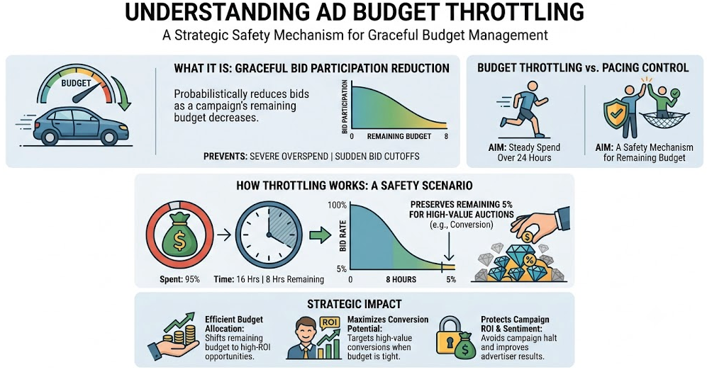
Budget throttling is the process of gracefully reducing bid participation as a campaign's remaining budget decreases, preventing severe overspend or sudden bid cutoffs that would halt a campaign mid-day. Unlike pacing control (which aims for steady spend over 24 hours), throttling is a safety mechanism: when a campaign has spent 95% of its daily budget with 8 hours left, throttling probabilistically reduces the bid rate to preserve the remaining 5% for high-value auctions.

The challenge is subtle but critical. A naive approach—"if remaining budget < 5%, bid in 10% of auctions"—causes severe bid suppression cascades: if multiple campaigns hit their budget ceiling simultaneously (e.g., at 3 PM on a Friday), the exchange's overall bid volume plummets, CPMs spike for publishers, and user experience degrades. A better approach uses feedback: each bidder observes its own bid acceptance rate and spend velocity, then adjusts its throttle probability smoothly to avoid discontinuous drops.

The business impact is twofold. First, throttling prevents runaway overspend: a campaign with a $100k daily budget that accidentally hits $102k overspend (2%) loses $2k and potentially violates advertiser contracts. Second, throttling preserves auction quality: instead of a hard cutoff at 100%, a smooth reduction from 100% bid rate at 90% spend to 10% bid rate at 99% spend gives the exchange time to route impressions to other campaigns, maintaining competitive dynamics and CPM stability.

Key challenges include: (1) latency—throttle decisions must be made in < 5ms, ruling out expensive computations; (2) coordination—across a fleet of bidders, all throttle probabilities must increase or decrease together to avoid wild swings in exchange volume; (3) feedback stability—the throttle mechanism must not oscillate (spend bounces between high and low); (4) fairness—campaigns with identical budgets and remaining spend must face identical throttling, regardless of which bidder processes their auction.

Scale considerations: a hyperscale exchange has thousands of campaigns in the throttle zone simultaneously. At 100k QPS, ~5k campaigns might be at 90%+ spend at any moment. Each requires a decision every 10–50ms. Central coordination becomes difficult; local decision-making is necessary.

Key Requirements

Functional Requirements

• Proportional throttling: As remaining budget decreases, bid probability decreases (e.g., 100% at 90% spend, 50% at 95% spend, 10% at 99% spend).
• Per-campaign thresholds: Support configurable throttle curves (e.g., aggressive for some campaigns, conservative for others).
• Smooth transitions: No cliff edges (where bid probability drops from 90% to 10% in one step); ensure gradual reduction.
• Overspend safeguard: If a campaign exceeds 100% of budget, reject all subsequent bids until the next pacing cycle.
• Multi-currency support: Some campaigns are budgeted in USD, others in EUR or JPY; throttle probabilities must account for exchange rates.
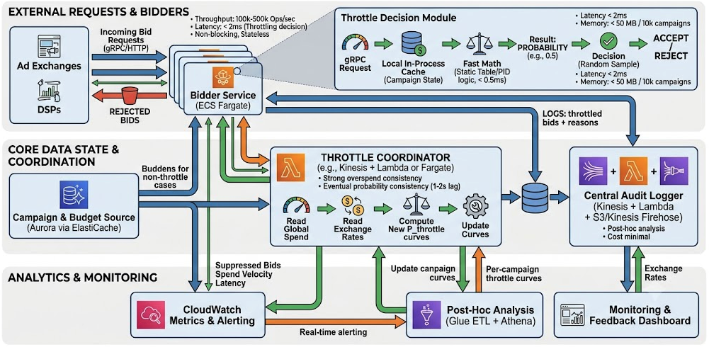
• Audit logging: Log every throttled bid decision (suppressed + reason) for post-hoc analysis.

Non-Functional Requirements

• Throttle decision latency: < 2ms (pure in-process math, no external calls).
• Throughput: Support 100k–500k 'compute throttle probability' operations per second.
• Consistency: Strong consistency for budget overages (once overspent, immediately reject bids); eventual consistency for throttle probability (may lag by 1–2 seconds).
• Cost: Minimal; throttling logic should not require external services.
• Memory: < 50 MB per 10k campaigns (campaign_id, spend, budget, throttle_state).
• Availability: 99.99% uptime for throttle logic (graceful fallback to no throttling acceptable).

Simplified Architecture

Architecture Proposals

Option 1: Static Threshold Ladder with ECS In-Process State

Divide the budget spend range into discrete brackets, each with a fixed throttle probability. For example:

• 0–80% spent: bid probability = 100%
• 80–90% spent: bid probability = 90%
• 90–95% spent: bid probability = 50%
• 95–99% spent: bid probability = 10%
• 99%+ spent: bid probability = 0% (reject all)

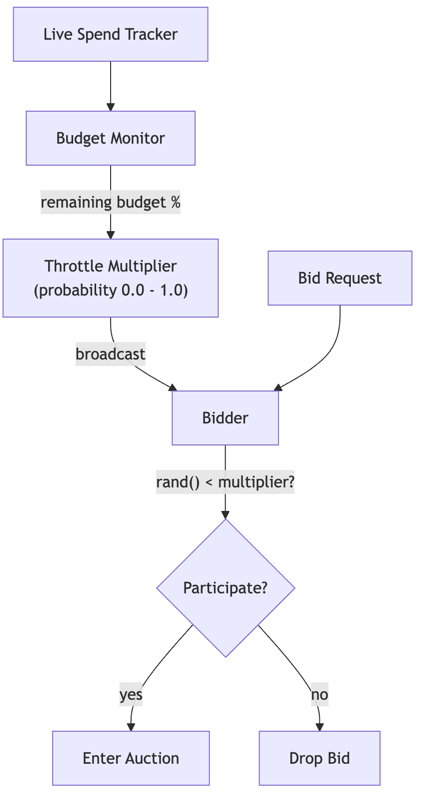
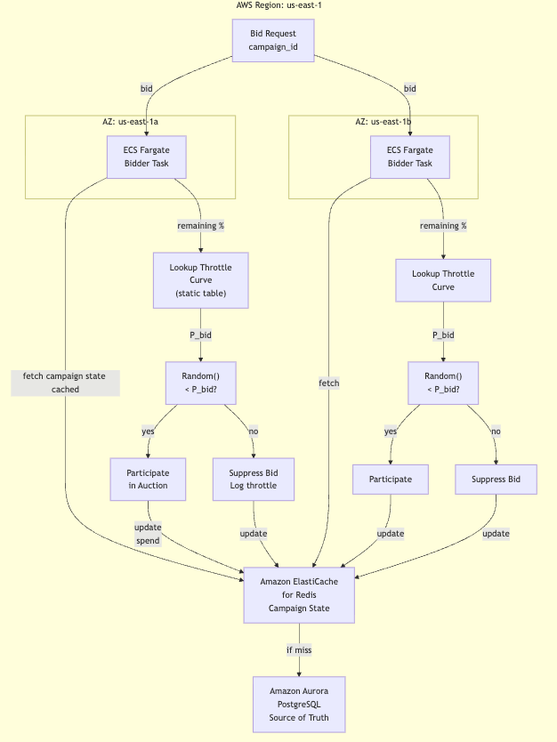
On each bid request, the bidder computes remaining_budget / total_budget, finds the corresponding bracket, and makes a probabilistic decision. Campaign state is cached locally (with periodic refreshes from Amazon Aurora via ElastiCache).

Why it works:

• Extremely simple: a table lookup and a random number generation.
• Deterministic: same budget level always produces the same probability (no oscillation).
• No central coordination: each bidder independently applies the curve.
• Campaign state is cached in ElastiCache with Aurora as source of truth.

Pros:

• Low latency: pure in-process; likely < 0.5ms.
• Easy to understand and tune: operators can visualize the curve and adjust bracket boundaries.
• No external dependencies: works even if central services fail (falls back to cached state).
• Minimal memory overhead: just a static lookup table (16 entries max) + cached campaign state in ElastiCache.
• ElastiCache TTL ensures fresh state within seconds.

Cons:

• Static thresholds do not adapt to traffic patterns: if traffic drops mid-day, campaigns underspend and never enter throttle zones; if traffic spikes, campaigns overspend rapidly. The fixed curve is suboptimal for both scenarios.
• Cliff edges at bracket boundaries: at 89% spend with P=90%, a bid is likely accepted; at 90.1% spend with P=50%, it is likely rejected. Users may notice a sudden drop in impression volume. Mitigate by overlapping brackets or using a continuous curve instead.
• No feedback: the curve does not adjust based on actual observed bid acceptance rates, which vary by publisher, time of day, and user segment. A campaign might be designed to have 100% spend but only 80% of its budget is actually available (e.g., low-quality inventory is rejected by the advertiser's quality filter).
• Unfairness under concurrent bidders: multiple bidders competing for the same user might all apply the throttle probability independently, causing accidental coordination (e.g., if two bidders both suppress 90% of bids for a campaign, the campaign only participates 1% of the time instead of 10%).

Failure Modes & Mitigations:

• Brackets tuned for average traffic; traffic is 5x higher than expected: Campaigns exhaust budget 5x faster, triggering throttle at earlier spend percentages. Mitigate by monitoring real-time spend velocity via CloudWatch and alerting if it deviates > 20% from forecast.
• Curve causes undershoot (campaign has 50% budget remaining at day-end): Thresholds are too conservative; campaigns spend < 100% of budget. Mitigate by making brackets more aggressive (move bracket boundaries earlier) or reducing bid suppression probability per bracket.
• ElastiCache cache miss or network partition: Bidders cannot fetch fresh campaign state. Mitigate by using a local in-process cache with a fallback to conservative throttling (assume worst case if state is stale).

When to Choose: Choose Option 1 for small systems (< 1k campaigns, < 10k QPS) where simplicity is paramount. Also useful as a fallback mechanism in more complex systems: if the main throttle system fails, revert to Option 1.

Option 2: PID Controller with Kinesis Feedback Loop

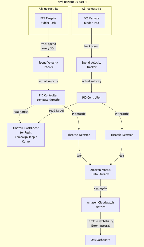
Instead of static brackets, use a PID feedback loop (similar to Option 3 in pacing control) to continuously adjust the throttle probability based on observed spend velocity vs. target spend curve. ECS Fargate bidders track spend; Kinesis aggregates and broadcasts adjustments.

How it works:

1. Campaign target curve: For a $1,000 daily budget, the target is $41.67/hour. Bidders track actual spend every 10–30 seconds.
2. Throttle probability computation: P_throttle = P_base - K_p * error - K_i * integral_error - K_d * derivative_error, where error = (target spend velocity - actual spend velocity).
3. When error is positive (actual spend > target), the controller increases throttle probability (reduces bids). When error is negative (actual spend < target), it decreases throttle probability (accepts more bids).
4. The derivative term (K_d) prevents oscillation by dampening rapid changes.
5. PID state is stored in ElastiCache; updates are published to CloudWatch Metrics for monitoring.

Why it works:

• Adaptive: responds in real-time to deviations from target, automatically adjusting for traffic spikes.
• Smooth: integral and derivative terms prevent oscillation and sharp transitions.
• Flexible: works with any target curve (linear, exponential, custom).
• Decentralized: each bidder independently runs its own PID controller; no central coordination needed.

Pros:

• Automatic adaptation: no tuning of bracket boundaries; the controller tunes itself based on observed error.
• Smooth transitions: no cliff edges; throttle probability changes gradually.
• Accounts for feedback: if actual spend differs from target, the error term drives the system back to equilibrium.
• Resilient: continues working even if global spend patterns change unexpectedly.
• Observable: every bidder logs its P_throttle, error, and integral via CloudWatch for monitoring.

Cons:

• Requires tuning of K_p, K_i, K_d parameters. Poor tuning causes oscillation (P_throttle bounces between high and low, causing bid volume to ping-pong) or overshoot (campaign spends > budget before controller catches it).
• Delayed response: the integral term accumulates error over time, introducing lag. If spend velocity changes suddenly, the controller takes 5–10 seconds to react.
• Complex monitoring: operators must understand control theory to debug issues. If a campaign is oscillating, should K_d be increased or K_p decreased? The answer depends on detailed analysis.
• Requires synchronization: all bidders must agree on the target curve (which hour are we in?) and the controller tuning parameters. Clock skew introduces systematic errors.

Failure Modes & Mitigations:

• K_p is too high: P_throttle overshoots; campaign overspends by 5–10% before the derivative term damps the response. Mitigate by reducing K_p or increasing K_d (dampening).
• Clock skew causes all bidders to misestimate spend velocity: If system time drifts 10 seconds, all bidders report identical errors, and the controller applies throttling simultaneously. Mitigate by using server-provided canonical time from ElastiCache or NTP.
• Controller diverges due to integral windup: The integral term accumulates errors until P_throttle is 0 or 1 (saturated). Once saturated, the controller cannot correct. Mitigate by capping the integral term (e.g., integral error <= 100, preventing runaway accumulation).
• Kinesis replication lag: Audit metrics lag behind actual throttle decisions. Mitigate by using local CloudWatch PutMetric calls instead of Kinesis for real-time visibility.

When to Choose: Choose Option 2 for systems with variable traffic patterns or campaigns that have non-linear spend targets (e.g., campaigns that ramp spend over time). Requires a team comfortable with control theory and willing to invest in tuning and monitoring.

Option 3: ML-Driven Contextual Bandit with SageMaker

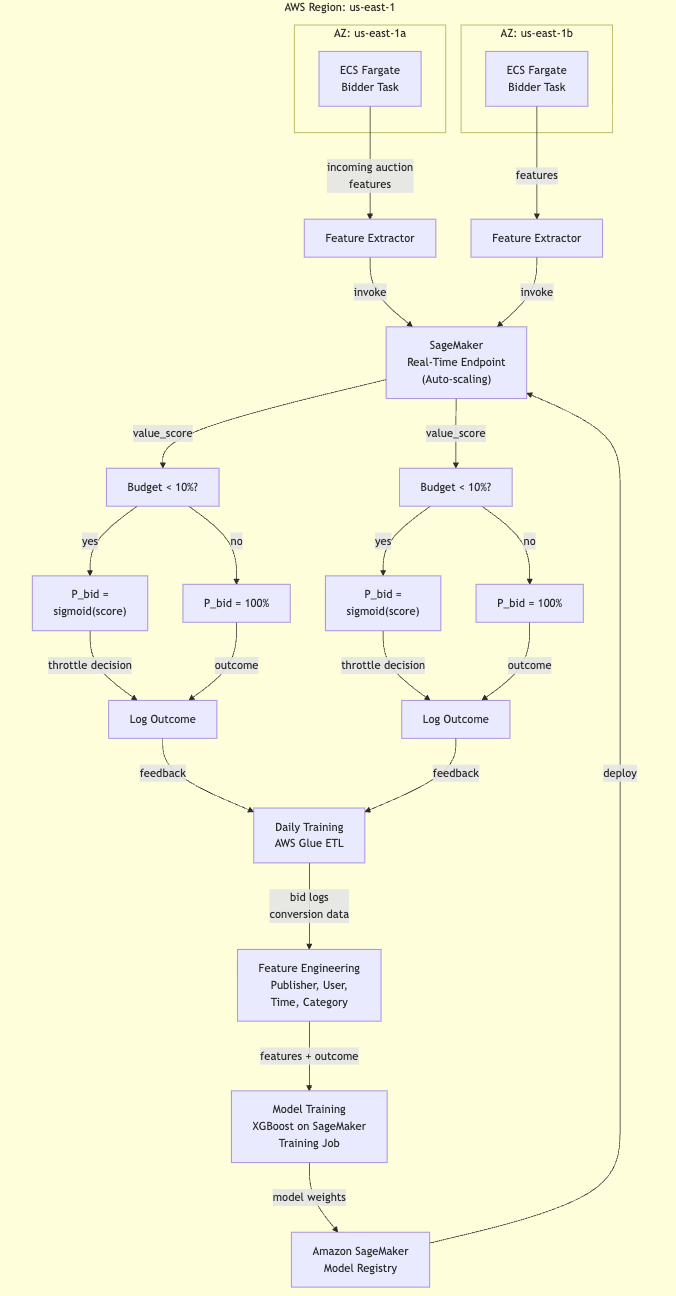
Instead of deciding "bid or not" based solely on remaining budget, train a machine learning model to predict which auctions have high conversion value. When budget is tight, prioritize auctions with predicted high ROI. Model inference runs via Amazon SageMaker (real-time endpoint or serverless async endpoint) behind an internal Network Load Balancer.

How it works:

1. Training (daily): For each auction, collect features (publisher, user context, time of day, category) and the outcome (bid won? converted?). Train a regression model: value_score = model(features).
2. Model serving: SageMaker Real-Time Endpoint (auto-scaling behind NLB) or Serverless Async Endpoint. Bidders call the endpoint via gRPC or HTTP.
3. Online throttling: When a campaign is in the throttle zone (remaining budget < 10%), compute value_score for the incoming auction.
4. Throttle decision: P_bid = sigmoid(value_score - threshold). High-value auctions (high value_score) have P_bid > 50%; low-value auctions have P_bid < 10%.
5. Learn and adapt: Periodically (hourly), retrain the model using the latest performance data via AWS Glue ETL job.

Why it works:

• Value-aware: prioritizes high-ROI auctions, maximizing spend efficiency even under budget constraints.
• Learns from data: the model improves over time as it observes which auctions actually convert.
• Graceful degradation: if the model is unavailable, fall back to Option 1 (static thresholds).
• SageMaker handles scaling and serving; bidders simply invoke the endpoint.

Pros:

• Maximizes campaign ROI: instead of arbitrarily suppressing 90% of bids when budget is tight, it suppresses low-value bids, ensuring the remaining budget is spent on high-quality impressions.
• Adapts over time: the model automatically learns seasonal patterns, publisher performance differences, and user segment behaviors.
• Handles non-linear budget curves: can model complex relationships between features and value that static thresholds cannot capture.
• SageMaker auto-scaling ensures latency remains low even during traffic spikes.

Cons:

• High operational complexity: requires ML infrastructure (SageMaker, feature store, model registry), data science expertise, and continuous monitoring for model drift.
• Latency: feature extraction + model inference adds 5–20ms to bid latency (usually acceptable, but not sub-millisecond like Options 1 and 2). Mitigate with SageMaker Serverless Endpoints for bursty workloads.
• Training data bias: if the training data is skewed (e.g., overrepresents high-value auctions), the model will overestimate value. Requires careful data preprocessing and bias detection.
• Feedback loops: if the model suppresses low-value auctions, it may never see performance data for them, preventing the model from learning their true value. Requires exploration strategy (occasionally bid on "suppressed" auctions to collect feedback).
• Model staleness: retraining hourly is expensive; if you retrain daily, the model is 12+ hours stale during peak hours and may not reflect real-time auction value changes.

Failure Modes & Mitigations:

• Model overfits to training data: Performs well on historical auctions but poorly on new patterns. Mitigate by using cross-validation, regularization (L1/L2), and monitoring prediction error on live data via SageMaker Model Monitor.
• Feature drift: A feature used in training (e.g., "publisher reputation score") changes definition or calculation, causing model predictions to diverge from reality. Mitigate by versioning features and monitoring their distributions (data quality checks via Great Expectations).
• SageMaker endpoint latency spikes: During traffic surges, model inference queues up. Mitigate by configuring SageMaker Autoscaling with aggressive scale-up policies or using Serverless Async Endpoints for non-real-time throttling.
• Feedback loop exploitation: A competitor trains a similar model and learns which auctions your campaign values most; they preemptively bid higher on those auctions. Mitigate by adding noise to throttle decisions or occasionally bidding on low-value auctions to confuse competitors.

When to Choose: Choose Option 3 for large, mature exchanges (thousands of campaigns, billions of daily impressions) where maximizing ROI under budget constraints is a competitive advantage. Requires a data science team and ML infrastructure investment (3–6 months to build and tune).

Comparison Table

Recommendation

For startups and small exchanges (< 1k campaigns, < 10k QPS): Use Option 1 (Static Thresholds). Implement a simple lookup table with 5–10 brackets. Adjust brackets quarterly based on observed spend patterns. This requires < 1 week of development and no ongoing maintenance beyond threshold tuning.

For mid-market exchanges (1k–10k campaigns, 10k–100k QPS): Start with Option 1, then transition to Option 2 (PID Controller) once you have operational experience with throttling. Option 2 is a better long-term solution for adaptive systems. Invest 2–3 weeks in PID implementation and tuning via CloudWatch metrics; the payoff is smoother spend curves and less manual threshold adjustment.

For hyperscale exchanges (10k+ campaigns, 100k+ QPS) or ROI-critical scenarios: Consider Option 3 (ML-Driven Bandit) as a parallel system that coexists with Option 1 or 2. For high-value campaigns (top 10% by spend), use Option 3 to maximize ROI; for long-tail campaigns, use Option 1 for simplicity. This hybrid approach requires ~6 months to implement but yields significant ROI improvements (3–8% revenue lift is typical).

For all options:

• Implement comprehensive monitoring via CloudWatch of throttle decisions: log every suppressed bid, compute the overall suppression rate, and alert if it deviates > 20% from expected.
• Validate that throttle decisions are fair: campaigns with identical budget and remaining spend should have similar suppression rates, regardless of which bidder processes their auction. Use statistical tests (chi-squared goodness-of-fit) to detect unfairness.
• Run A/B tests before deploying new throttle logic: compare Option 1 vs. Option 2 on a subset of campaigns for 1–2 weeks, measure spend variance and revenue lift, then roll out.

Capacity & Performance Notes

Sizing for a hyperscale exchange:

• 100k bids per second
• 50k active campaigns
• Average daily budget: $20k per campaign
• Throttle zone (remaining budget < 10%): ~5k–10k campaigns active at any moment

Option 1 (Static Thresholds):

• Campaign state per bidder: 50k campaigns × (8 bytes campaign_id + 8 bytes spent + 8 bytes budget + 4 bytes timestamp) = 1.4 MB per bidder. With 20 bidders, ~28 MB total. Negligible.
• ElastiCache: cache.t4g.small (1 GB, ~$20/month). TTL set to 30 seconds; frequent refresh from Aurora ensures freshness.
• Lookup latency: O(1) table lookup via bracket index = ~0.1 microseconds.
• Memory for threshold table: 10 brackets × 2 floats (lower bound, probability) = 80 bytes. Negligible.

Option 2 (PID Controller):

• Campaign state per bidder: spent + budget + velocity + error_integral + P_throttle. ~60 bytes per campaign. 50k campaigns × 60 = 3 MB per bidder. With 20 bidders, ~60 MB. Negligible.
• Compute latency: velocity calculation (subtract two floats), error calculation, PID math (multiply-add for 3 terms). ~10–20 microseconds. < 1ms even at 500k QPS.
• Kinesis: 4 shards, on-demand pricing (~$100/month). Aggregation Lambda: < 100 MB memory, ~$50/month.
• Tuning parameters: K_p = 0.1, K_i = 0.01, K_d = 0.05 (typical starting values). Simulate offline to determine final values.

Option 3 (ML-Driven Bandit):

• Feature extraction: 20–50 features per auction (publisher_id, user_segment, category, hour_of_day, etc.). Feature computation + caching: ~1 microsecond if cached, ~100 microseconds if computed per auction.
• Model inference: Linear regression (50 features × 50 weights + bias + sigmoid): ~5 microseconds on CPU, < 1 microsecond on GPU.
• SageMaker Real-Time Endpoint: auto-scaling (2–10 instances of ml.c5.xlarge, ~$500–$2k/month). Latency p99 ~20ms including network round-trip.
• Model size: 50k features × 8 bytes = 400 KB (negligible). Feature cache (if hot features are cached): ~100 MB.
• Training cost: offline job on Spark/Glue. 1B bid logs (1 day of bids) × 50 features = 50 GB raw data. Training XGBoost: ~30 minutes on a 10-core machine. Retraining daily costs ~$100/month (compute + storage).

Example throttle curves:

Option 1 (static):

Spend % | P_bid
0–80    | 100%
80–90   | 90%
90–95   | 50%
95–99   | 10%
99+     | 0%

Option 2 (PID):

At 85% spent (target 83%): error = +0.02
P_throttle = 0.5 - 0.1 * 0.02 - 0.01 * (accumulated error) - 0.05 * (change in error)
          = 0.5 - 0.002 - 0.0005 - 0.001
          = 0.497 (slight throttle)

Option 3 (ML):

For a high-value auction (value_score = 3.5):
P_bid = sigmoid(3.5 - 2.0) = sigmoid(1.5) = 0.82 (high probability)

For a low-value auction (value_score = 0.5):
P_bid = sigmoid(0.5 - 2.0) = sigmoid(-1.5) = 0.18 (low probability)