Ad Indexing at Hyperscale: 100,000 Campaigns in Under 5ms

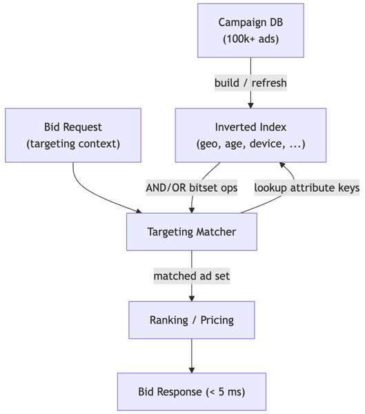
Ad indexing is the process of selecting which campaigns to bid for given a user's profile and context. Given 100,000+ active campaigns, each with targeting predicates (e.g., "show only to users aged 18–35 in the US, on Chrome, interested in travel"), a bidder must identify matching campaigns in under 5 milliseconds. An incorrect index can cause catastrophic failures: if the index misses matching campaigns, reach is lost; if it returns non-matching campaigns, invalid bids waste budget.

The technical challenge is extraordinary: 100,000 campaigns × 20 attributes per campaign (gender, age range, geo, device type, interest categories) = 2 million predicate evaluations per auction, which would consume 200+ milliseconds. Real systems must prune the search space through indexing: using carefully constructed data structures (inverted indices, decision trees, or bit vectors) to eliminate non-matching campaigns before evaluating expensive predicates.

The business impact is direct: faster ad indexing means lower latency end-to-end (improving user experience and CPM), and more complete campaign coverage (higher revenue). A 1ms improvement in indexing latency can improve exchange-wide latency by 20%, and incomplete indexing can leave 5–20% of bidding potential on the table.

Key challenges include: (1) predicate complexity—campaigns use AND/OR logic ("age 18–35 AND (interests: travel OR interests: luxury)"), requiring efficient boolean filtering; (2) frequent updates—campaigns are added, paused, or removed every second, necessitating online index rebuild; (3) memory constraints—a naive in-memory index of all 100k campaigns × 20 attributes could consume 100+ GB; (4) latency tail—p99 index lookups must stay below 10ms even during traffic spikes.

Scale considerations: hyperscale exchanges handle 100k–500k bid requests per second. Each bid request triggers a single index lookup. That is 100k–500k index queries per second. An index that takes 2ms per query would require 200–1,000 dedicated index servers just to keep up; clearly, indexes must be in-process (sub-millisecond) or heavily cached.

Key Requirements

Functional Requirements

• Exact predicate matching: Return all campaigns whose targeting rules match the incoming user context (no false positives or false negatives).
• Complex predicates: Support AND, OR, NOT logic (e.g., "(age 18–35) AND (geo: US OR geo: CA) AND NOT (device: Android)")
• Fast updates: Add, remove, or modify campaigns without rebuilding the entire index (< 100ms latency).
• Result ranking: Return campaigns in priority order (e.g., by bid floor, brand importance, or historical fill rate).
• Coverage metrics: Track how many campaigns match each user context (for business reporting).

Non-Functional Requirements

• Index lookup latency: < 5ms p50, < 10ms p99 (time spent searching the index, not including network or other operations).
• Throughput: Support 100k–500k 'query index' operations per second.
• Memory footprint: < 1 GB for 100k campaigns on a single bidder instance (aggressive compression required).
• Update latency: < 100ms for adding/removing a campaign (rebuild index or update data structure).
• Consistency: Strong consistency for active campaigns (no race conditions); eventual consistency for dormant or paused campaigns (ok to service stale state for a few seconds).
• Availability: 99.99% uptime for index queries (fallback to historical campaign set acceptable).

Simplified Architecture

Architecture Proposals

Option 1: In-Memory Roaring Bitmap Inverted Index with S3 Distribution

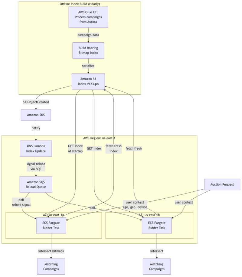
Build a Lucene-style inverted index: for each targeting attribute value (e.g., "age: 25–34", "geo: California"), maintain a Roaring Bitmap (compressed integer set) of campaign IDs that include that value. Campaign index is built offline via AWS Glue, stored on Amazon S3, pulled by bidder ECS tasks at startup, and updated via S3 event notifications → Amazon SNS → ECS task reload signal.

How it works:

1. Index construction (AWS Glue job): For each attribute value, store a Roaring Bitmap of campaign IDs.
   • Example: index["age:25-34"] = Roaring([1002, 3045, 5001, 7234, ...])
   • Roaring Bitmaps compress dense sequences efficiently (e.g., [1000–1100] stored as a range, not 100 individual integers).
2. Query (user in age 25–34, in California, on desktop):
   • Look up index["age:25-34"] → Roaring([1002, 3045, 5001, ...])
   • Look up index["geo:CA"] → Roaring([1001, 1002, 3000, 3045, ...])
   • Look up index["device:desktop"] → Roaring([1000, 1001, 1002, 3000, ...])
   • Intersect all three: [1002, 3045] (campaigns matching all three predicates)
3. Complex predicates (AND/OR): Build a small query plan tree and evaluate recursively.
4. Index distribution: Build index → S3 → bidder ECS task pulls at startup; on S3 PUT event → SNS → Lambda → signal ECS task to reload.

Why it works:

• Roaring Bitmaps are highly optimized for compression and fast intersection (CPU cache-friendly bitwise operations).
• Inverted index is a proven data structure; Lucene and Elasticsearch use variants.
• Scales gracefully: even with 100k campaigns, a Roaring Bitmap uses ~50–100 KB per attribute value.
• S3 storage decouples index building from bidder serving; safe, versioned updates.

Pros:

• Sub-millisecond lookups: Roaring bitmap intersection is O(k) where k is the smaller set size (usually < 1,000 campaigns).
• Memory efficient: Roaring Bitmaps compress repetitive patterns. 100k campaigns across 1,000 attribute values = ~50 MB total (vs. 500 MB for naive hash maps).
• Handles complex predicates: AND/OR/NOT logic translates to bitmap union, intersection, and complement operations.
• S3-backed: immutable index versions, versioning, cheap storage ($0.023/GB/month).
• Atomic updates: ECS tasks reload the entire index via SQS signal, avoiding partial-load race conditions.

Cons:

• Complex predicate parsing: translating natural language predicates (e.g., "age AND (interest_1 OR interest_2)") into bitmap operations requires careful query planning.
• Offline updates introduce lag: if a campaign is added/paused/removed, it takes 1 hour (Glue job interval) before bidders see the change. For time-sensitive campaigns, unacceptable. Mitigate with online incremental updates or more frequent Glue jobs.
• Stale data: if a campaign is paused but still in the index, a query will return it (false positive). Requires a separate "active campaigns" filter applied post-index-lookup (check campaign status in Aurora or ElastiCache).

Failure Modes & Mitigations:

• Roaring Bitmap corruption during build: Glue job crashes mid-write, corrupting S3 index file. Mitigate by writing to temp file first, then atomically moving to final location. Validate index integrity (checksums) before bidders consume.
• Memory explosion if attribute cardinality is high: If a campaign targets 10,000 unique ZIP codes, the index grows proportionally. Mitigate by grouping predicates (e.g., store "regions: [NW, SW, NE, SE]" instead of "zipcodes: [98101, 98102, ...]") or using a secondary filter.
• Slow intersection if multiple bitmaps are large: If 10,000 campaigns match "age:25–34" and 10,000 match "geo:US", intersection takes time. Mitigate by pre-sorting bitmaps by cardinality (small first) and early-stopping if an intermediate result is empty.

When to Choose: Choose Option 1 for hyperscale exchanges with stable campaign sets (< 10% churn per day). The index is mature and well-understood, making it a safe choice for production systems.

Option 2: Decision-Tree / Range-Tree Hybrid Index with Aurora Backing

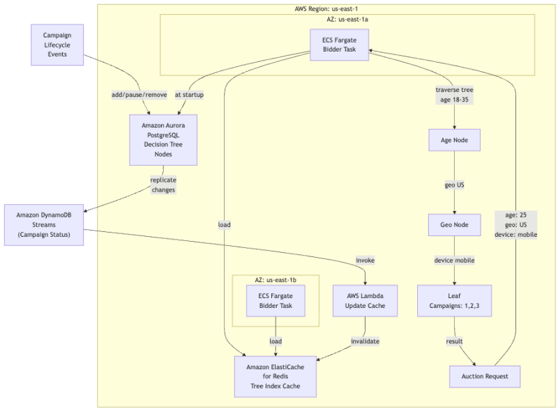
Build a multi-dimensional decision tree where each level partitions the search space along one attribute. For example: level 1 partitions by age (buckets: 0–17, 18–35, 36–55, 55+); level 2 partitions by geo (states); level 3 by device type. Tree nodes are stored in Amazon Aurora (PostgreSQL with JSON columns) for easy updates and strong consistency.

How it works:

1. Index construction: Build tree top-down in Aurora. Each node contains a list of campaigns matching that node's subtree.

   Root
   ├── Age 0–17
   │   ├── Geo: US
   │   │   ├── Device: mobile → [Campaign 5, 10, 12]
   │   │   └── Device: desktop → [Campaign 5, 20]
   │   └── Geo: EU
   │       └── Device: mobile → [Campaign 15]
   ├── Age 18–35
   │   ├── Geo: US
   │   │   └── Device: mobile → [Campaign 1, 2, 3, 100, 101]
   │   ...
   

2. Query traversal: For each user attribute, descend the tree, eliminating subtrees that don't match.
   • User age 25: descend to "Age 18–35" node.
   • User geo US: descend to "Geo: US" node.
   • User device mobile: descend to "Device: mobile" leaf node.
   • Result: [Campaign 1, 2, 3, 100, 101].
3. Range queries: For continuous attributes (age, price), use interval trees to efficiently find overlapping ranges.
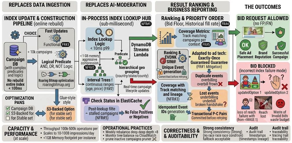
4. Caching: Bidders load the tree from Aurora at startup, cache it in ElastiCache with 30-second TTL, and subscribe to DynamoDB Streams for real-time campaign lifecycle updates (add/pause/remove).

Why it works:

• Tree traversal is O(depth × branching factor), usually 3–5 levels and 2–10 branches per level = 10–100,000 operations per query, but with excellent cache locality.
• Range queries are efficient: interval trees answer "which campaigns target age 25–34?" in O(log N + K) where K is the result size.
• Supports hierarchical attributes naturally: "geo: US > states > counties > ZIP codes" is a natural tree structure.
• Aurora provides strong consistency and ACID transactions for updates.

Pros:

• Intuitive model: tree structure mirrors how humans think about targeting (age bracket → geo region → device type).
• Fast range queries: interval trees are O(log N + K), beating naive scans.
• Memory efficient: campaigns are stored once at the deepest matching node, not duplicated across nodes.
• Handles attribute dependencies: if age is correlated with device choice (teens prefer mobile, seniors prefer desktop), the tree structure naturally captures this via subtree organization.
• Real-time updates: Aurora changes propagate via DynamoDB Streams to Lambda, which invalidates ElastiCache entries.

Cons:

• Tree imbalance: if one attribute has high cardinality (e.g., 1M ZIPcodes) and another has low cardinality (e.g., 2 genders), the tree may be deep and unbalanced, hurting lookup speed. Requires careful attribute ordering (low-cardinality first).
• Complex updates: inserting a new campaign with a complex targeting rule (e.g., "age 25–45 OR geo: EU") requires careful tree traversal and potential restructuring. Easy to introduce bugs.
• Range overlaps: if campaigns target overlapping age ranges (one targets 18–35, another targets 25–45), the tree must store both, leading to duplication and complexity.

Failure Modes & Mitigations:

• Tree becomes unbalanced: All campaigns are in subtrees under "Device: mobile" because that is the dominant device type. Tree is deep, lookups are slow. Mitigate by monitoring tree depth via CloudWatch and rebalancing (rebuild from scratch) weekly if depth > 8.
• Range query misses: If a campaign targets age "25 ≤ age < 35" and you query for age 34, an imprecise range tree may miss it. Mitigate by storing ranges as closed intervals [25, 34] and using careful inequality checking.
• Aurora scaling: At 100k campaigns, tree rebuild can take seconds. Mitigate with Aurora read replicas (one per region) and caching via ElastiCache.

When to Choose: Choose Option 2 when targeting predicates are highly hierarchical and attribute values have natural groupings (geo by region, age by decade, etc.). Also useful when the system expects frequent range queries (e.g., price bucketing).

Option 3: Vectorized GPU Scan with EC2 GPU Instances

Instead of indexing, store campaigns in a columnar format (one column per attribute) and use SIMD or GPU operations to parallelize the filtering. For each incoming auction, scan all campaigns in parallel, evaluating predicates in vectorized fashion. Suitable for very large campaign sets (> 500k).

How it works:

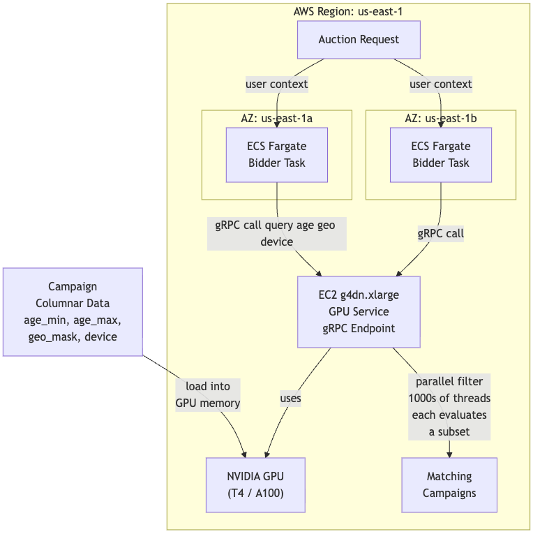
1. Columnar storage: Store campaigns in a layout optimized for SIMD scans on GPU.

   campaign_ids:   [1,      2,      3,      ...]
   age_min:        [18,     13,     21,     ...]
   age_max:        [35,     18,     55,     ...]
   geo_mask:       [0x03,   0x01,   0xFF,   ...]  (bitmask: bit i set if campaign targets region i)
   device_type:    [0x05,   0x01,   0x03,   ...]  (bitmask: bits 0=mobile, 1=tablet, 2=desktop)
   

2. Query vectorization: For a user (age: 25, geo: region 1, device: mobile):
   • Evaluate age_min <= 25 AND 25 <= age_max for all campaigns in parallel (SIMD).
   • Evaluate geo_mask & (1 << region) != 0 for all campaigns in parallel.
   • Evaluate device_type & MOBILE_BIT != 0 for all campaigns in parallel.
   • AND the three boolean results across all campaigns.
3. GPU acceleration: If campaigns are numerous (>100k), offload scanning to GPU (NVIDIA T4 or A100). GPU can evaluate millions of predicates per second.
4. Deployment: EC2 instance with GPU (g4dn.xlarge or p4d.24xlarge) runs a gRPC service that handles predicate queries. ECS Fargate bidders call the gRPC service.

Why it works:

• SIMD and GPU are purpose-built for data-parallel workloads; filtering thousands of campaigns simultaneously is their bread and butter.
• Columnar layout maximizes cache efficiency: iterating over a single column (e.g., age_min for all campaigns) keeps the CPU cache hot.
• Scales gracefully: if you have 10x more campaigns tomorrow, simply allocate 10x more GPU memory and threads; the algorithm is unchanged.

Pros:

• Fastest possible: GPUs can evaluate ~1B predicates per second, making even 1M campaigns instantaneous.
• Simple logic: no complex indexing; just scan and filter. Easier to implement correctly and debug.
• Scales with hardware: buy a better GPU, queries get faster proportionally.
• Handles complex predicates naturally: bitmasks and bitwise operations are GPU-native.

Cons:

• GPU cost and power consumption: high-end GPUs cost $5k–$15k and consume 250–400W. Not economical for small exchanges.
• gRPC latency: querying a remote GPU service adds 1–5 microseconds per query. Acceptable for batch queries, problematic for single auctions.
• Not great for sparse workloads: if only 10% of campaigns are active, you are still scanning all 100%. Index-based approaches skip inactive campaigns.
• Predicate expressiveness: complex, non-linear predicates (e.g., "IF age < 25 THEN prefer device=mobile ELSE prefer device=desktop") are hard to vectorize.

Failure Modes & Mitigations:

• GPU out of memory: Campaign set grows beyond GPU VRAM. Mitigate by splitting campaigns across multiple GPUs or using CPU-GPU streaming (process campaigns in chunks).
• gRPC service overload: Too many queries, service cannot keep up. Mitigate by batching queries (process 100 auctions together) to amortize gRPC latency or auto-scaling the GPU instance count.
• SIMD lane divergence: Some campaigns match, some don't; divergence causes unused GPU threads. This is acceptable (GPUs handle it gracefully), but severely unbalanced predicates can reduce efficiency.

When to Choose: Choose Option 3 only if you have a large, stable campaign set (>500k) and can afford GPU hardware and operational complexity. Suitable for very large DSPs or Google-scale systems. Not recommended for most ad exchanges.

Comparison Table

Recommendation

For startups and small DSPs (< 10k campaigns, < 10k QPS): Use Option 1 (Roaring Bitmap Inverted Index). Build a simple index using a library (e.g., roaringbitmap.org). Spend 2–3 weeks implementing; this is the safest, most battle-tested approach. Store index on S3 for easy distribution.

For mid-market exchanges (10k–100k campaigns, 10k–100k QPS): Use Option 1 with optimizations: prune inactive campaigns (every 6 hours), batch updates (accumulate new campaigns for 1 minute, rebuild index once), and implement a secondary "active campaigns" filter in ElastiCache to handle paused campaigns without full index rebuilds. This gives you 95% of the benefits of Option 2 at 1/5 the complexity.

For large exchanges with hierarchical predicates (100k+ campaigns, 100k+ QPS): Consider Option 2 (Decision Tree) if your predicates have natural hierarchical structure (geo by country/state/county, demographics by age bracket). Invest 4–8 weeks to build and tune tree balancing logic. Expect 2–5ms lookups. Use Aurora for strong consistency and DynamoDB Streams for real-time updates.

For hyperscale systems with extreme latency requirements (< 1ms p99): Use Option 3 (GPU Scan) only if (1) campaign set is very large (> 500k) and stable, (2) you have GPU hardware available, and (3) you have a team comfortable with CUDA/GPU programming. This is a 3–6 month project and should be treated as a core infrastructure investment.

Hybrid approach: Many large exchanges use Option 1 for 95% of campaigns and Option 2 (or even sequential scan) for the remaining 5% of high-targeting campaigns. This balances simplicity with coverage.

For all options, implement comprehensive campaign coverage metrics: log the number of matching campaigns per auction, grouped by campaign stage (active, paused, archived). Alert if coverage drops (indicating index bugs or stale data).

Capacity & Performance Notes

Sizing for a hyperscale exchange:

• 100k campaigns
• 500k bids per second
• 30 attributes per campaign on average
• 50 distinct values per attribute (on average)

Option 1 (Roaring Bitmap Inverted Index):

• Index size: 30 attributes × 50 values = 1,500 entries. Each entry is a Roaring Bitmap with ~100 campaign IDs on average = 1,500 entries × 1 KB per bitmap = 1.5 MB. Plus campaign metadata (campaign_id, bid_floor, priority): 100k × 32 bytes = 3.2 MB. Total: ~5 MB per bidder instance.
• Lookup time: 3–5 attribute lookups (age, geo, device, interest, etc.) × 100 microseconds per bitmap intersection = 300–500 microseconds = 0.3–0.5ms. P99 with contention: ~2ms.
• Update latency: Glue job runs hourly; index rebuild takes 5 minutes. New campaigns appear in the index within 1 hour. For faster updates, run Glue every 10 minutes (~$50/month extra cost).

Option 2 (Decision Tree):

• Tree size: depth 4–5 levels, branching factor 3–5. Worst case: 5^4 = 625 leaves. Each leaf contains ~160 campaigns on average = 625 leaves × 160 × 8 bytes = 800 KB. Plus internal nodes (pointers, thresholds): ~1 MB. Total: ~2 MB per bidder instance.
• Lookup time: 4–5 tree traversals × 1 microsecond per node (pointer dereference, comparison) + bitmap intersection at leaf = 5 + 100 = ~105 microseconds = 0.1ms. P99: ~1ms.
• Update latency: inserting a campaign may require tree rebalancing. If tree is balanced with B-tree-style rebalancing, insert is O(log N) = O(17) node operations. ~500 microseconds. But full tree rebuild (weekly) takes ~5 minutes on Aurora.

Option 3 (Vectorized GPU Scan):

• Columnar data: 100k campaigns × 30 attributes × 4 bytes (int32 or bitmask) = 12 MB. Fits easily in GPU VRAM (typical NVIDIA GPU has 8–40 GB).
• Lookup time: broadcast user context to GPU (1 microsecond gRPC latency), launch kernel (0.1 microsecond GPU dispatch), scan 100k campaigns with 1,000 CUDA threads (100 campaigns per thread × 10 cycles per filter = 1,000 cycles = 2 microseconds at 500 MHz GPU clock). Total: ~10 microseconds. P99: ~20 microseconds.
• Throughput: 500k QPS / (10 microseconds per query) = needs GPU that can process 5k queries/microsecond. A modern GPU processes ~1 trillion ops/sec = 1M queries/microsecond (if using 1k ops per query). Plenty of headroom.
• Memory on GPU: 12 MB campaign data + 1 MB working memory per 1k concurrent queries = 12 + 500 = ~512 MB for 500k QPS. Easily fits.