Ad Impression Forecasting (aka Ad Inventory Forecasting): Architecting for Scale, Speed, and Accuracy

Inventory forecasting predicts the volume of available ad impressions (by inventory segment, geography, device, daypart) that a publisher will have available in the future—hours to weeks ahead. Accurate forecasts are essential for yield optimization, budget allocation, and deal pricing. Publishers use forecasts to set reserve prices (too high and they waste cheap inventory; too low and they leave money on the table); bidders use forecasts to allocate daily budgets across publishers (if ESPN.com will have 50M sports impressions tomorrow, they reserve budget accordingly); programmatic guaranteed deals rely on forecasts (buyer commits to 10M impressions at $8 CPM; seller must forecast supply to ensure 10M inventory is available).

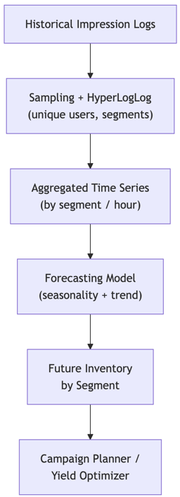
The technical challenge is volume and variance. Large publishers generate billions of impression logs daily (one row per impression, with timestamp, content metadata, segment ID, viewability flag). Naive forecasting—querying the full log and applying a time-series model—requires hours of batch compute per day, is too slow for real-time budget allocation decisions, and consumes massive network bandwidth. Instead, systems use sampling and cardinality estimation techniques: HyperLogLog approximates unique inventory segment values; sampling retains ~1% of impressions and applies statistical models to that sample. This reduces data volume by 100x, enabling fast, near-real-time forecasting in <10 minutes.

Further complexity arises from temporal patterns. Inventory volume varies by hour (primetime > off-peak), day of week (weekday ≠ weekend), season (holidays, summer doldrums), and external events (sports tournaments, news crises). A naive ARIMA or Prophet model trained on last-30-days data will miss holiday spike patterns if holidays are rare. Advanced systems use feature engineering (day-of-week, is-holiday, is-major-event flags) and ensemble methods to capture these patterns.

At the largest scale (YouTube, Google Ad Manager, Amazon Publisher Services), forecasting must operate across 100M+ distinct inventory segments (publisher×country×content-category×device-type×daypart combinations), billions of daily log events, and extreme variance (some segments have <100 impressions/day, others >10M). Naive approaches (one time-series model per segment) become 100M-fold computational burden.

Key Requirements

Functional Requirements

• Forecast available inventory volume (impressions) per segment (publisher, geography, device, daypart) for 1 hour to 30 days ahead
• Support multiple forecast horizons: real-time (next hour), daily (next 7 days), weekly (next 4 weeks)
• Predict with >90% accuracy (MAPE <10%) for high-volume segments (>100k impressions/day)
• Handle spiky/high-variance segments gracefully: for <10k impressions/day segments, provide ranges (10th, 50th, 90th percentiles) instead of point estimates
• Detect and adjust for holidays, major events, and anomalies
• Support drill-down: forecast total impressions, then break down by country/device/daypart
• Provide feature importance: help ops understand which factors drive forecasts (seasonality, day-of-week, trend, etc.)
• Retrain forecasts multiple times daily; serve latest predictions via API with <500ms latency

Non-Functional Requirements

• Throughput: generate forecasts for 10M segments multiple times/day (~100 billion predictions/day total)
• Latency: serve forecast query (1 segment, multiple horizons) in <500ms (p99)
• Data freshness: retrain models using data available as of <1 hour ago
• Accuracy: MAPE <10% for segments with >100k impressions/day; <25% for smaller segments
• Storage: archive forecasts and actuals for 2 years (audit, learning, improvement)
• Scalability: linear increase in infrastructure with number of segments; no algorithmic bottlenecks
• Operational observability: alert if forecast accuracy degrades >2 percentage points vs. historical baseline via CloudWatch

Simplified Architecture

Architecture Proposals

Option 1: HyperLogLog + Prophet/ARIMA Batch Pipeline

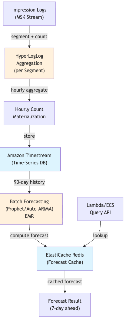
This option uses HyperLogLog cardinality estimation to summarize daily impression volumes, then feeds summary statistics to a time-series forecasting model (Prophet or auto-ARIMA). HyperLogLog is a probabilistic data structure that counts distinct values using minimal memory (~1 KB per segment for 1 billion unique values).

Workflow: (1) Ingestion: Streaming pipeline (Amazon MSK) processes impression logs; for each segment, a HyperLogLog sketch is updated incrementally. Every hour, sketch is materialized to a count (e.g., today's volume = 5.2M impressions for segment ESPN.com / US / sports / mobile / primetime). (2) Aggregation: Batch job (hourly, runs on Amazon EMR in ~10 minutes) aggregates HyperLogLog counts across all segments into a time-series database (Amazon Timestream or RDS Timescale). (3) Forecasting: Prophet or auto-ARIMA model is fitted per segment using 90-day historical data (from Timestream). Forecast for next 7 days is computed and cached in ElastiCache Redis. (4) Serving: API (Lambda or ECS) queries cache; serves forecast in <10ms.

Pros:

• Extremely cheap: HyperLogLog requires <1 KB per segment; MSK stream processing is stateless and highly parallelizable
• Fast: batch aggregation runs in ~10 minutes on EMR; forecasting in <5 minutes; entire pipeline 15 minutes end-to-end
• Battle-tested: Prophet (Facebook) and auto-ARIMA are production-grade time-series libraries
• Approximate but acceptable: HyperLogLog provides ~1% error margin on cardinality; acceptable for forecast inputs
• Operational simplicity: no complex ML infrastructure; standard Python + Spark jobs on EMR
• Explainability: Prophet outputs trend, seasonality, holiday components; easy to debug why forecast is high/low

Cons:

• Coarse granularity: daily volumes only; cannot forecast hourly variation (must assume intraday pattern from historical average)
• Limited feature engineering: Prophet is primarily trend + seasonality; adding custom features (ad spend, competitor activity) is difficult
• Segment cardinality explosion: 100M segments requires 100M forecasting jobs; even at 1 second per job, total time is ~27 hours (more than a day)
• Recency bias: last-7-days pattern may not be representative (especially for seasonal content); requires careful holdout tuning
• Cold-start segments: new segments with <7 days history get poor forecasts; must fall back to heuristics

Failure Modes & Mitigations:

• HyperLogLog hash collision: Sketch undercounts true volume by 5–10%. Mitigation: Use conservative sketch size (16 KB, <1% error); validate sketch accuracy quarterly by comparing to exact count on high-volume segments.
• Seasonal pattern not learned: Prophet model trained on last 90 days misses yearly seasonality (e.g., Christmas peak). Mitigation: Include external regressors (is_holiday, day_of_year); use yearly seasonality period (365 days) if available.
• Outlier spike: New ad campaign drives 10x volume spike; forecast jumps 10x. Mitigation: Manually flag spike as anomaly via Lambda; refit model excluding spike day; use robust loss functions (Huber loss) less sensitive to outliers.

When to Choose: Use this option if you have a large publisher (10M+ daily impressions, 100k+ segments) and want predictable, low-cost forecasting. Fast retraining (15 min) enables daily forecast updates. Acceptable accuracy for most yield management use cases. Operational overhead is minimal: standard batch pipeline on EMR + SQL queries on Timestream.

Option 2: Spark/Flink Batch over Parquet Logs with LightGBM

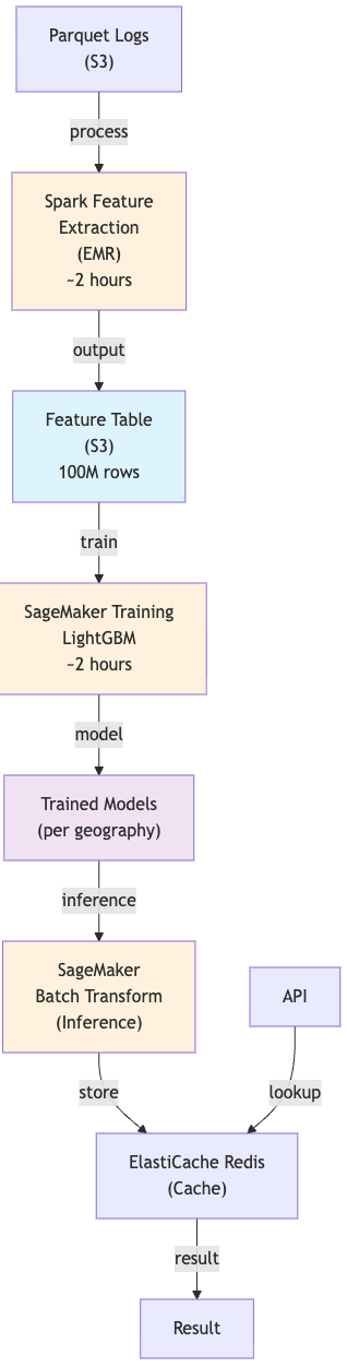
This option trades HyperLogLog's approximation for exactness and richer features. Instead of sampling/cardinality estimation, the system periodically re-processes the full impression log (Parquet, in object storage) using Spark or Flink, extracts features per segment (volume, trend, day-of-week effect, content category, geo patterns), and trains a gradient-boosting model (LightGBM, XGBoost) to predict next-period volume.

Workflow: (1) Daily batch ingest: Parquet logs from yesterday are written to S3. (2) Feature extraction (Spark job on EMR, ~2 hours): Process full Parquet log; compute per-segment statistics (daily volume last 90 days, trend slope, day-of-week deviation, seasonality indicators, competitor spend). Output feature table: 100M rows × 20 columns to S3. (3) Model training (SageMaker, ~2 hours): Split data into train/validation; train LightGBM model with features predicting next-period volume via SageMaker training jobs. Output: 1 model per geography (e.g., US, EMEA, APAC). (4) Batch inference: SageMaker Batch Transform scores all segments; results cached in ElastiCache. (5) Serving: API queries cache.

Pros:

• Exact counts: no approximation error from HyperLogLog; 100% accurate input data
• Rich features: model can learn complex patterns (e.g., "sports content has 20% higher volume on Sundays"; "news spikes during elections")
• High accuracy: gradient-boosting often achieves <5% MAPE on high-volume segments
• Transferable: single model trained per geography serves all segments (vs. one model per segment)
• Feature importance: LightGBM outputs which features drive predictions; explainability for ops
• Handles cold-start better: model can extrapolate for new segments using similar historical segments

Cons:

• Computational cost: Spark jobs run 4–6 hours daily on EMR; SageMaker training adds cost
• Latency to forecast: full retraining takes 6+ hours; forecasts are stale (based on yesterday's data)
• Storage overhead: Parquet logs + feature table + models consume ~100 TB monthly (for large publishers)
• Operational complexity: Spark/Flink job management on EMR, model versioning via SageMaker, monitoring multiple models
• Overfitting risk: model trained on last 90 days may not generalize if patterns shift (seasonality, consumer behavior)
• Scalability: linear in data volume; 100B daily impressions → 100M feature rows → requires large EMR cluster

Failure Modes & Mitigations:

• Model overfitting: Model achieves 95% accuracy on validation set but forecasts poorly on new data (pattern shift). Mitigation: Use time-series cross-validation on EMR (train on days 1–80, validate on days 81–90); monitor out-of-sample MAPE daily via CloudWatch; retrain if accuracy drops >2%.
• Missing holidays: Model trained on last 90 days doesn't include major holiday; forecast misses next holiday season. Mitigation: Manually add holiday features (is_holiday, days_to_holiday) in feature extraction; curate a holiday calendar in DynamoDB external to data.
• Data quality: Some segments have data corruption (e.g., one day shows 1000x volume spike due to logging bug). Mitigation: Implement data validation in Spark job: flag segments with >5x median daily change as anomalies; filter from training.

When to Choose: Use this option if you have engineering resources to maintain Spark/Flink pipelines on EMR and want highest accuracy forecasts. Payoff is 5–10% improvement in forecast accuracy vs. Option 1, leading to better reserve prices and yield optimization. Requires data engineering team; not suitable for small publishers.

Option 3: Streaming Forecast with Online Learning (Flink + River)

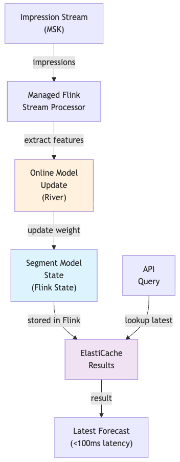
This option implements continuous forecasting: as new impression data streams in (real-time, via MSK), the system updates forecasts incrementally without waiting for daily batch jobs. Uses stream processing (Amazon Managed Service for Apache Flink) paired with online learning library (River, or TensorFlow's online learning APIs) to fit models incrementally.

Workflow: (1) Streaming ingestion: Impressions flow into MSK partitioned by segment. (2) Online model update (Managed Flink): For each segment, maintain an online learning model (e.g., online gradient descent, mini-batch SGD). As each micro-batch of impressions arrives, the model is updated with new data via Flink state. (3) Continuous inference: At any moment, a segment's latest model can be queried for tomorrow's forecast; no waiting for batch jobs. Results written to ElastiCache. (4) Serving: API queries latest model; returns forecast in <100ms.

Pros:

• Real-time forecasts: as soon as new data arrives, forecasts are updated; no waiting for nightly batch
• Responsive to change: if volume pattern shifts mid-day, forecast adapts within hours
• Cost-effective: continuous job runs at low parallelism (only one model per segment); CPU-light on Flink
• Accuracy on dynamic patterns: online learning naturally handles concept drift (e.g., if ad spend increases, model adapts)
• Cold-start good: model trains on first few days of data; can serve forecasts before 90-day window
• Explainability: River outputs model coefficients/feature weights incrementally via CloudWatch

Cons:

• State management complexity: maintaining 100M online models in Flink state is operationally hard (state recovery, checkpointing to S3)
• Instability: online learning models can oscillate or diverge if learning rate is poorly tuned; may produce wild forecasts
• Less powerful than batch: online learning sacrifices some accuracy for speed (mini-batch models < full-batch models)
• Feature engineering limited: complex feature engineering (multi-day interactions, seasonal components) harder in online setting
• Debugging difficulty: online models evolve over time; hard to reproduce an issue from 3 days ago (state is lost)
• Scalability headache: checkpointing state for 100M models to S3 may require enormous storage / recovery time

Failure Modes & Mitigations:

• Model divergence: Learning rate too high; model oscillates and produces increasingly poor forecasts. Mitigation: Start with conservative learning rate in Flink job; monitor forecast MAPE per segment via CloudWatch; alert if >30% error; auto-reset model.
• State corruption: Flink crashes; state checkpoint to S3 is corrupted; model is unrecoverable. Mitigation: Dual-write models to S3 every 1 hour; fallback to batch model if state recovery fails.
• Concept drift: Volume pattern shifts (e.g., new content, competitor launch); old model is invalid. Mitigation: Detect drift via statistical test (e.g., Adwin algorithm in River); alert ops; optionally reset model to retrain.

When to Choose: Use this option if you have a streaming infrastructure team (Managed Flink operators), need forecasts to adapt in <6 hours to market changes, and can tolerate slightly lower accuracy for responsiveness. Ideal for dynamic inventory markets (programmatic guaranteed deals with daily inventory adjustments). Not recommended unless you are already running Managed Flink for other purposes.

Comparison Table

Recommendation

Start with Option 1 (HyperLogLog + Prophet) for any publisher with >10M daily impressions. It is fast to deploy on EMR, requires minimal infrastructure, and provides adequate accuracy for most yield optimization use cases (reserve price setting, budget allocation). Implement alerting on forecast accuracy via CloudWatch; if MAPE consistently >15%, move to Option 2.

Migrate to Option 2 (Spark + LightGBM) once you have >500M daily impressions and a dedicated data engineering team. The 5–10% accuracy improvement translates to measurable CPM gains (1–3% yield lift). Plan a 2–3 month migration: run Option 1 and Option 2 in parallel on EMR and SageMaker, compare forecasts on real impressions, and gain confidence in LightGBM before deprecating Prophet.

Adopt Option 3 (Online Learning) only if you operate in a fast-changing market (e.g., programmatic guaranteed deals with daily adjustments) or use forecasts to drive real-time decisions (minute-by-minute budget allocation). Requires Managed Flink expertise and careful tuning; not recommended for most publishers. Hybrid approach: use Option 2 as baseline via SageMaker, add Option 3 for fast-moving segments only.

For all options, maintain monitoring via CloudWatch:

• Daily MAPE per segment (aggregated by volume tier)
• Forecast vs. actual plots (are predictions biased high/low?)
• Feature importance analysis (what drives forecasts? Are patterns expected?)
• Anomaly detection (did today's actual volume exceed forecast's 90th percentile? Why?)

Capacity & Performance Notes

HyperLogLog + Prophet (Option 1):

• HyperLogLog size: 100M segments × 1 KB = 100 GB (fits on 2–3 high-memory ElastiCache nodes)
• Prophet training on EMR: 100M segments × 1 second = ~27 hours; mitigated by sampling (forecast only top 10M segments daily, others weekly)
• Forecast storage: 10M segments × 7 days × 4 bytes = 280 MB; cached in ElastiCache (single instance, 256 GB)
• Query latency: ElastiCache lookup <1ms; 500ms SLA comfortably met

Spark + LightGBM (Option 2):

• Feature table size: 100M segments × 90 days × 20 features × 4 bytes = ~72 GB on S3
• Spark job on EMR: 100 executors × 4 cores = 400 cores; 4–6 hours
• LightGBM training via SageMaker: single model per geography (US, EMEA, APAC); ~10 minutes per model
• Model size: 50 MB × 3 geographies = 150 MB; cache entire models in ElastiCache
• GPU acceleration: optional; 1 GPU (ml.g4dn.xlarge) can train all 3 models in parallel (1 model = 5 minutes)

Online Learning Streaming (Option 3):

• Managed Flink state size: 100M segments × model state (50 KB) = ~5 TB (distributed across Flink taskmanagers)
• State checkpoint size: 5 TB to S3 every 1 hour; requires 5 TB network bandwidth per hour (~11 Gbps sustained)
• Segment model latency: inference <50ms per model
• Throughput: Managed Flink can process 1M impressions/sec (100-node cluster); easily handles largest publishers

Accuracy Boundaries:

• Option 1: peaks at ~88% accuracy (MAPE 12%); Prophet's time-series modeling ceiling
• Option 2: achieves 94–96% (MAPE <5%) for high-volume segments; lower for long-tail (<10k/day)
• Option 3: 90–93% (MAPE 7%); slightly lower than batch due to online learning efficiency trade-off