The AI Powering Billions of Tailored Ads - Dynamic Creative Optimization

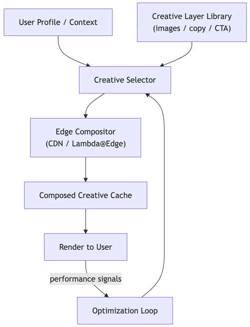
Dynamic Creative Optimization (DCO) automatically tailors each ad impression to the individual viewer by composing creative elements (image, headline, copy, call-to-action) based on user context (location, device, weather, time of day, inferred intent). Instead of a single fixed creative, the system generates billions of micro-tailored variants—each optimized for likelihood of click, conversion, or brand engagement. For an e-commerce advertiser (clothing, travel, automobiles), DCO can show different products to different viewers from the same campaign; a travel ad shows beaches to summer-seekers, mountains to adventure tourists, skiing to winter visitors—all from a unified creative template.

The business impact is significant: DCO typically drives 10–50% improvement in click-through rate (CTR) and 5–30% improvement in conversion rate over static creatives. At scale (1B impressions/day), even 5% CTR improvement translates to 50M additional clicks, worth millions in incremental revenue for advertisers. This makes DCO a high-value feature that drives advertiser adoption and loyalty.

The technical challenge is multi-faceted:

(1) Latency: composition must happen in <50ms as part of the RTB flow;

(2) Variant explosion: with N creative layers (3–5 typical) and K elements per layer (5–20 typical), the combinatorial space is K^N (if only 5 layers × 10 elements each = 100k combinations);

(3) Optimization: which variant maximizes CTR for user U given context C? Answering requires real-time learning (contextual bandits) or fast cache lookup of pre-computed best variants;

(4) Freshness: new creatives, new context signals, new audiences emerge constantly; system must adapt within hours, not days.

At scale (YouTube, Criteo, TradeDesk, Facebook), DCO runs on billions of impressions daily across diverse audiences. The system must handle both high-compute scenarios (render-on-demand composition when no cached variant exists) and cache-first scenarios (95% of composition hits a pre-computed cache, rendering in <5ms).

Key Requirements

Functional Requirements

• Dynamically compose creative by selecting and layering elements (image, headline, copy, CTA, color) based on user context
• Support context dimensions: geography, device type/size, weather, daypart, user segment, inferred intent, A/B test variant
• Generate and cache top-N creative variants per segment (e.g., top 5 variants for "US + mobile + age 25-34 + raining")
• Measure performance (CTR, conversion, brand lift) per variant and per context dimension
• Implement online learning (contextual bandits, Thompson sampling) to optimize variant selection toward maximizing conversion
• Support A/B testing: test new creative elements or algorithms in shadow mode before production
• Fallback gracefully: if composition logic fails, serve a safe default creative (house ad or last-known-good)
• Provide ops dashboards: show top-performing variants by segment, CTR trends, render latency distribution

Non-Functional Requirements

• Latency: compose and return creative in <30ms (p99) for cache hits; <100ms for cache misses
• Throughput: compose 100k–1M creatives per second across all geographies
• Cache hit rate: >95% (pre-computed variants serve majority of requests)
• Availability: 99.99% uptime; graceful fallback if DCO service unavailable
• Consistency: same user + same context must consistently see the best-performing variant (no flicker)
• Freshness: new creative elements indexed within 5 minutes; performance data (CTR) available within 1 hour
• Scalability: linear cost increase with number of creative variants; sub-quadratic with number of context dimensions

Simplified Architecture

Architecture Proposals

Option 1: Pre-Rendered Combinatorial Cache

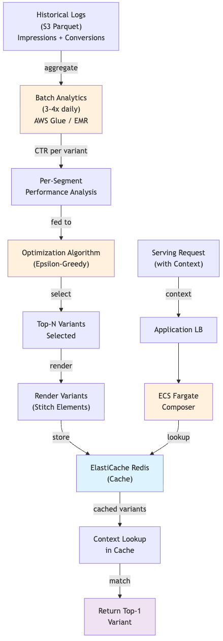
This option pre-computes and caches the top-N creative variants for each context segment. Offline batch job (daily or several times/day via AWS Glue or EMR) analyzes historical performance data (which variant got highest CTR for "US + mobile + age 25–34" segment in the last 7 days?), generates top-3 variants, renders them as static images or JSON templates, and stores in ElastiCache Redis. At serving time, request includes context (geo, device, user segment); ECS Fargate service looks up cached top-N variants for that context, returns the top-1 (or A/B tests between top-2).

Implementation: (1) Offline batch (runs 3–4x daily via Glue or EMR): Query impression + conversion logs from S3, aggregate by context segment, compute CTR/conversion rate per variant-segment pair using Spark. Run optimization algorithm (e.g., epsilon-greedy, upper confidence bound) to select top-N variants per segment. (2) Rendering: For each top-N variant, generate final HTML/JSON creative (stitch image, copy, CTA from S3); store in ElastiCache with key = hash(context_segment). (3) Serving: ECS Fargate request includes context (extracted from user data, real-time geo, device, weather API). Service computes context_hash, looks up ElastiCache, returns cached variant.

Pros:

• Extremely fast: cache hit returns in <5ms (ElastiCache lookup + template substitution)
• Deterministic: same context always gets same variant (no randomness, consistent UX)
• Simple operationally: no real-time ML required; batch pipeline is standard ETL via Glue
• Cost-efficient: no per-request compute; all expensive computation happens offline on EMR
• Safe: pre-computed variants are reviewed/QA'd before serving
• Easy to debug: "Why did user X see variant Y?" Answer: "Context matched segment S; variant Y was top-1 for S"

Cons:

• Coarse-grained optimization: optimizes per segment, not per individual (all users in "US + mobile + age 25–34" see same variant)
• Long tail underserved: segments with <1k daily impressions get poor optimization (sparse historical data)
• Adaptation lag: new creatives not reflected until next batch run; 3–4x daily batches = hours delay
• Combinatorial explosion: if context has 10 dimensions (geo, device, age, gender, intent, season, daypart, weather, A/B test, …), segment cardinality explodes (10^6 combinations); pre-computing top-N for all is expensive
• Wasted variants: top-N may not be top-1 by individual (segment average is not user-specific)
• Cold-start: new campaigns/creatives have no historical data; no variants to serve

Failure Modes & Mitigations:

• Cache miss: User context matches no pre-computed segment; service returns None. Mitigation: Hierarchical fallback (if exact match misses, try coarser segments: drop daypart, drop age range, etc.; eventual fallback to default creative).
• Stale cache: Variant cached Tuesday is outdated by Friday; CTR has dropped 20%. Mitigation: Set ElastiCache TTL (2–4 hours for fast-moving variants, 24 hours for stable); prioritize re-computing high-traffic segments more frequently via Glue scheduler.
• Segment cardinality explosion: Trying to pre-compute for all 10^6 possible contexts is infeasible. Mitigation: Focus on high-traffic segments (top 100k segments cover 80% of traffic); use fallback for long-tail.

When to Choose: Use this option if you have well-defined, stable audience segments and can afford to recompute variants 3–4x daily via Glue or EMR. Ideal for large publishers (YouTube, Facebook) with massive impression volume that justifies batch infrastructure. Also suitable if creatives are relatively stable (not changing every hour).

Option 2: Edge-Side Composition with Lambda@Edge / CloudFront Functions

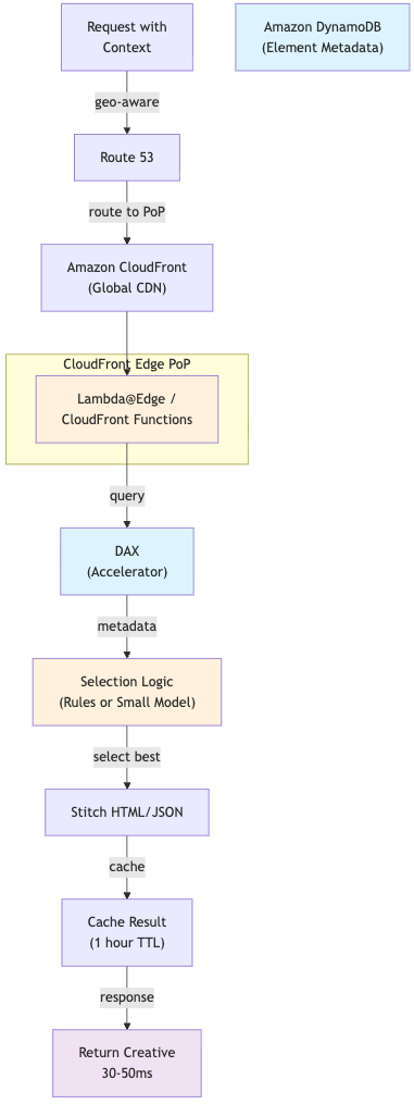
This option moves creative composition to the CDN edge, assembling variants dynamically at request time using lightweight serverless compute (AWS Lambda@Edge or Cloudflare Workers). No pre-computation; instead, the edge function receives a request, extracts context, looks up metadata (which images/copy elements are available?), selects the best combination, stitches them together, and returns the final creative within 30–50ms.

Implementation: (1) Element metadata service: Creative elements (images, headlines, copy, CTA buttons) are stored in a metadata database (Amazon DynamoDB or Firestore) with metadata (image URL, dimensions, copy text, conversion rate in last 7 days). Service is read-optimized for low-latency lookups. For speed, cache hot metadata in DAX (DynamoDB Accelerator) for sub-millisecond access. (2) Edge function: Lambda@Edge / CloudFront Functions queries metadata service, applies selection logic (e.g., "choose image with highest CTR for this geo"), stitches HTML/JSON response, caches result for 1 hour. (3) Composition logic: Implemented as a lightweight decision algorithm (rules engine or small model—not a 100 MB neural network; must fit in Lambda).

Pros:

• Per-user optimization: composition happens per request, can theoretically optimize for each individual user (not just segment average)
• Real-time responsiveness: new elements indexed and served within 1 hour (no batching delay)
• Scalability: edge compute distributes load; no central bottleneck
• Flexibility: composition logic can change without redeploying origin; update rules in DynamoDB metadata service
• Supports online learning: as new data arrives, metadata service updates element performance scores; edge logic immediately uses new scores
• Low cost: edge compute is pay-per-request; only active requests pay

Cons:

• Higher per-request latency: 30–50ms vs. 5ms for cached variants (6–10x slower)
• Cold-start: first request to new context has no cached result; full composition path is expensive
• Complexity: edge function must be stateless; cannot maintain model state or do complex computations
• Metadata service dependency: if DynamoDB/Firestore is slow or unavailable, compositions timeout
• Debugging difficulty: distributed across 50+ edge locations via CloudFront; hard to reproduce issues
• Security surface: edge function has access to user data, metadata service; potential injection/exfiltration risks

Failure Modes & Mitigations:

• Metadata service latency: DynamoDB lookup takes 50ms; composition times out. Mitigation: Cache metadata locally in Lambda/Worker memory (refresh every 1 hour); accept slight staleness for speed. Use DAX for sub-ms reads.
• Circular composition: Element selection logic chooses element A, which references element B, which references element A again. Mitigation: Validate composition logic offline; implement cycle detection in edge function; fallback to default if cycle detected.
• Element missing: Composition logic selects image that no longer exists (deleted from S3). Mitigation: DynamoDB metadata service validates element URLs on update; stale URLs are marked as unavailable in metadata.

When to Choose: Use this option if you want per-user optimization and have the engineering resources to manage Lambda@Edge and DynamoDB. Payoff is 1–5% additional CTR improvement over segment-based optimization. Ideal for large global platforms (Shopify, Airbnb, Uber) with diverse user bases and short time-to-market for new creative elements.

Option 3: ML-Driven Contextual Bandit with Online Learning

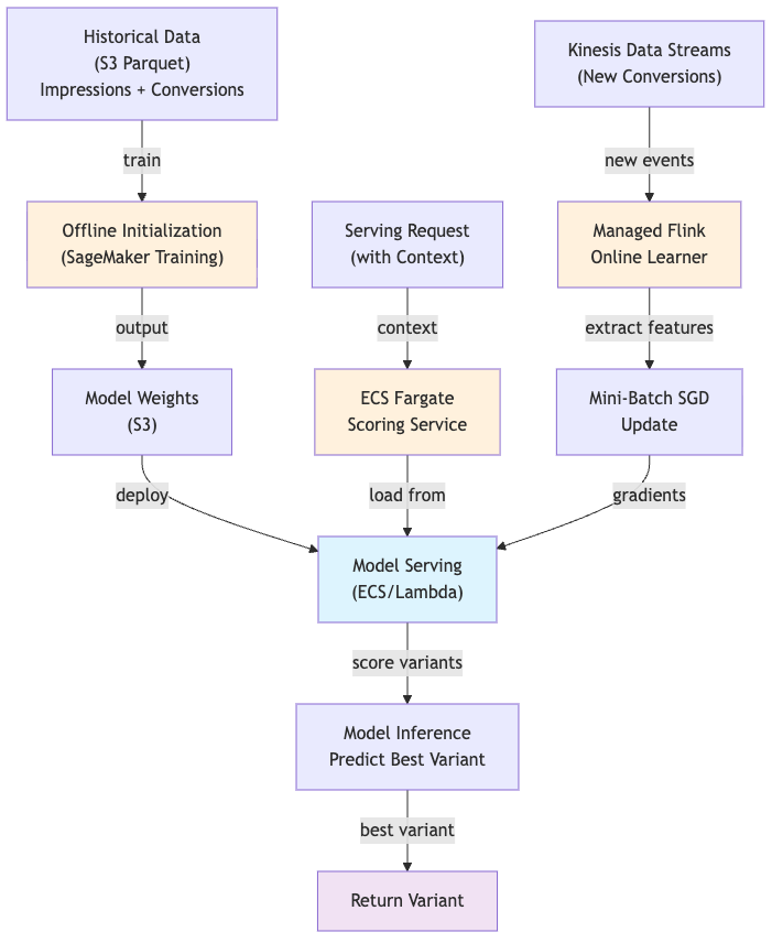
This option deploys an online learning system that continuously optimizes variant selection using contextual multi-armed bandit algorithms (Thompson sampling, upper confidence bound). A lightweight model is trained on-the-fly as impressions and conversions stream in, learning context-to-optimal-variant mappings. At serving time, the model predicts the best variant for the user's context.

Implementation: (1) Offline initialization: Batch job (daily) trains a contextual bandit model (e.g., linear Thompson sampling) on historical data using SageMaker, outputs model weights to a model serving infrastructure. (2) Online updates (Managed Flink Streaming or Kinesis): As new impressions and conversions arrive via Kinesis Data Streams, mini-batch updates are computed (compute gradient, apply SGD step) and pushed to model serving via ElastiCache or DynamoDB. (3) Serving: ECS Fargate request includes context; model scoring service (loaded from S3) predicts expected conversion for each variant, returns the best. Lightweight enough to run in <20ms. (4) Exploration: Bandit algorithm balances exploitation (choose best known variant) vs. exploration (try new variants to learn their performance); ensures freshness.

Pros:

• Optimized for individual users: model learns context-specific patterns (not just segment averages)
• Online learning: continuously improves as new data arrives; no batching delay
• Exploration-exploitation trade-off: bandit algorithm naturally tries new variants without explicit A/B test logic
• Data efficiency: learns quickly with small historical samples (better for long-tail creatives)
• Adaptability: if user behavior patterns shift (seasonality, trends), model adapts in hours
• Theoretical optimality: Thompson sampling, UCB are provably optimal in the long run

Cons:

• Operational complexity: must manage model training pipeline via SageMaker, model serving infrastructure, online updates
• Latency: model inference adds 20–30ms; slower than cache lookup
• State management: bandit model state evolves over time; must checkpoint and version in DynamoDB
• Exploration overhead: by design, the algorithm serves suboptimal variants ~10% of the time to explore; short-term CTR hit
• Debugging hard: why did the model choose variant X? Requires inspecting model weights and context encoding
• Cold-start poor: bandit learns slowly for very new creatives; may take days to find optimal variant

Failure Modes & Mitigations:

• Model divergence: Model weights explode or NaN due to learning rate too high or bad data. Mitigation: Clip gradients in Flink/Kinesis pipeline; validate weight magnitudes via CloudWatch (alert if >10x baseline); restart model if weights explode.
• Context encoding mismatch: Model trained on day 1 with context [geo, device]; new context dimension added on day 8 (weather). Mitigation: Versioned context schemas in DynamoDB; model predicts with only known dimensions; periodically retrain via SageMaker to incorporate new dimensions.
• Exploration regret: Bandit explores too much; CTR drops 5% as it tries bad variants. Mitigation: Use contextual Thompson sampling (more conservative exploration); set exploration rate explicitly (epsilon = 5%); monitor CTR weekly via QuickSight.

When to Choose: Use this option if you have an ML engineering team comfortable with online learning and can tolerate short-term CTR trade-off for exploration. Ideal for platforms where user behavior changes rapidly (news, social media, real-time events) or creatives are constantly evolving. Payoff is long-term optimization (5–10% CTR improvement) and fast adaptation to market changes.

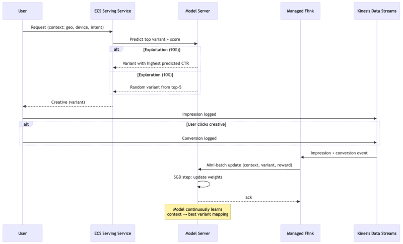
Option 3 (continued): Sequence Diagram for Online Learning with Exploration

This diagram shows how the contextual bandit system handles exploration and exploitation:

Comparison Table

Recommendation

Start with Option 1 (Pre-Rendered Cache) for any advertiser or publisher launching DCO. It is fast to implement (4–6 weeks), requires no ML infrastructure, and delivers 10–15% CTR improvement immediately. Invest in a good segment taxonomy (geography, device, audience, daypart); the quality of segments directly impacts optimization. Use AWS Glue for batch pipeline.

Migrate to Option 2 (Edge Composition) once you have >100M daily impressions and want to support rapid creative iteration (new elements, tests). Edge composition enables per-request customization without ML complexity; payoff is 15–25% CTR improvement. Requires partnership with Amazon CloudFront and DynamoDB engineering. Use DAX for ultra-fast metadata lookups.

Adopt Option 3 (Contextual Bandit) if you have an ML team and want maximum long-term optimization (20–40% CTR improvement). Ideal for data-driven advertisers (e-commerce, SaaS) where conversion value is high enough to justify continuous learning infrastructure via SageMaker and Managed Flink. Start with Thompson sampling (simpler than deep RL); monitor exploration overhead (CTR dip during learning phase); use bandit for new campaigns/creatives where historical data is sparse.

For all options:

• Measure lift via holdout A/B tests: DCO variant vs. control (single best creative)
• Monitor composition latency and fallback rates via CloudWatch; alert if either degrades
• Store all compositions and outcomes in audit log in S3 (for attribution, legal review)
• Respect creative constraints (brand guidelines, compliance); enforce at composition time

Capacity & Performance Notes

Pre-Rendered Cache (Option 1):

• Variant storage: 100k context segments × 3 variants × 50 KB/variant = 15 GB; fits on single ElastiCache instance (256 GB)
• Batch job via Glue/EMR: aggregate logs (5–10M impressions) by segment, compute CTR per variant (5 minutes), select top-N (2 minutes), render (5 minutes) = ~15 minutes total
• Fallback chain: exact segment → drop daypart → drop age range → drop intent → default creative (up to 5 fallbacks)
• Throughput: ElastiCache serves 500k QPS (single node); 5-node cluster = 2.5M QPS

Edge Composition (Option 2):

• Metadata service: 10k–100k creative elements × 10 KB metadata = 100 MB–1 GB in DynamoDB; cached in DAX for <1ms reads
• Edge function latency: DAX lookup 2ms + composition 20ms + cache write 5ms = ~27ms p99
• Throughput: Lambda@Edge handles millions of concurrent requests; auto-scales via CloudFront
• Cold-start: first request to new context triggers full composition (~40ms); subsequent requests cache hit within 5ms

Contextual Bandit (Option 3):

• Model size: linear model (context features × variant ids) = 1k features × 100 variants × 8 bytes = 800 KB per model; fits in memory
• Model inference: 20ms per request (feature extraction 10ms, scoring 10ms) on ECS Fargate
• Training throughput: Managed Flink processes 1M impressions/sec; SGD updates weights in mini-batches (10k impressions = 100ms)
• Exploration cost: 10% of traffic serves suboptimal variant; short-term CTR loss ~0.5–1% (recovered by long-term learning)

Scaling Boundaries:

• Option 1: segment cardinality ceiling at ~1M (beyond requires hierarchical fallback)
• Option 2: element count ceiling at ~10k (beyond requires DynamoDB sharding + DAX coordination)
• Option 3: feature count ceiling at ~10k (high-dimensional bandits converge slowly)